Bayes From Scratch, Part 1: Computing the Posterior Mean using Grid Search

I think the best way to learn new statistical methods is to code them myself from scratch. Crack open the papers and books, read the formulas, and build my own software. I don't plan on making software for release, this is a learning exercise. Here is the roadmap of some things I want to figure out in Bayesian statistics:

• Grid search posterior mean
• Grid search posterior regression
• Highest Posterior Density Interval
• Metropolis-Hastings algorithm for Markov Chain Monte Carlo
• Evaluating convergence (Rhat, $\widehat{R}$ and effective sample size, EFF)
• Multilevel models
• Hamiltonian MCMC

I feel like if I can code those things from scratch I will have a much better understanding of the problems that come up with convergence, or how to interpret results.

The data

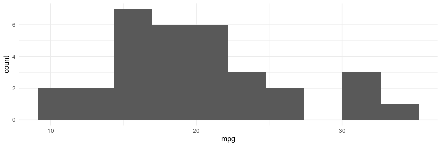
For this, I'm doing a super boring dataset that's built into base-R datasets library: mtcars.   I'm going to compute the mean miles-per-gallon using my prior understanding of what the average miles per gallon should be. So here's the data, there are 32 cases, a mean of 20.09 and median of 19.20.

Grid Search

In Richard McElreath's book^[1] he demonstrates estimating the posterior density of the proportion of the Earth that's covered in water. Kruschke's book^[3] also does an example with a binomial distribution with one parameter. I quickly realized why they chose this approach rather than computing a Bayesian mean. For a binomial density estimate you only need to know the number of attempts, the number of successes, and the probability of success. Thus it's pretty simple. The data is two numbers and you only have one parameter. But to compute the posterior mean you need two parameters the mean, $\mu$, and the standard deviation, $\sigma$, and the data is the vector of all the measurements of the variable.

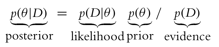
It wasn't clear to me about how to adapt  grid search to two parameters from one. The focus of only one parameter left me with a misconception. Because of the very simple introductions I was reading I thought maybe the $\theta$ in ye olde Bayes rule, seen below, was a single parameter. But it represents all the parameters in the entire model.

So here is the model I'm going to estimate. The $mpg$ is normally distributed with a mean of $m$ and a standard deviation of $s$. And I have defined some prior distributions for $m$ and $s$ that I discuss m

$$
mpg \sim Normal(m, s) \\
m \sim Normal(13, 3) \\
s \sim Uniform(0, 20)
$$

Following in McElreath's path (Rethinking, pg 40), we're going to take the grid search steps he outlined, with some minor modifications.

1. Define a grid. All the possible combinations of parameters we might want to use in estimating a posterior all laid out in a grid.
2. Compute the value of the prior for each pair of parameter values on the grid
3. Compute the likelihood at each pair of parameter values.
4. Compute the unstandardized posterior at each pair of parameter values by multiplying the prior and likelihood.
5. After all that, we standardize the posterior by dividing each value by the sum of all values

So let's just start with what the grid looks like. It's 100 values between 1 and 100 for the mean. And 100 values between 0.1 and 10 for the standard deviation. Already we are showing some of the downsides of this approach. There are only two parameters, and I'm only taking 100 values, but already this table has 10,000 rows ($100 \times 100$). Also what range should we reasonably choose for the values? These are arbitrary decisions. There are some reasonable values for it, but the values should represent what we expect to be the very extremes of the posterior.

N <- 100
g <- expand_grid(m = seq(1, 100, length.out = N),
            s = seq(0.1,10, length.out = N))

> head(g)
# A tibble: 6 x 2
      m     s
  <dbl> <dbl>
1     1   0.1
2     1   0.2
3     1   0.3
4     1   0.4
5     1   0.5
6     1   0.6

Priors

Bayesian statistics deviates from classical, frequentist statistics in a very key way - it considers prior knowledge of the systems we are studying as part of its calculation.  The choice of the prior can be from any information you may have prior to examining the data.

The priors have some good information. I choose a mean of 18 for the prior mpg because I had a car that regularly had 18 miles per gallon (now I live in the UK where that would be horrible, but it was somewhat common in the US). A frequentist approach would ignore prior knowledge about how the real world would work. For instance, without having any real values of fuel economy, we know that miles-per-gallon won't be negative. So our prior in this case greatly reduces the chances of seeing that.

mpg_m_prior <- dnorm(g$m, mean = 18, sd = 3)
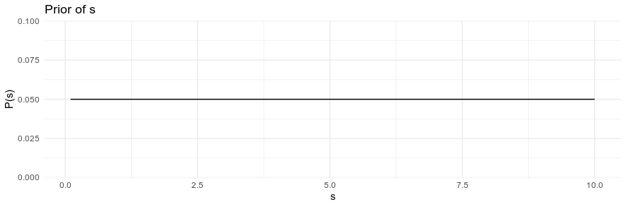
mpg_s_prior <- dunif(g$s, min = 0, max = 20)

The prior density is computed for every value of m and s in the grid.

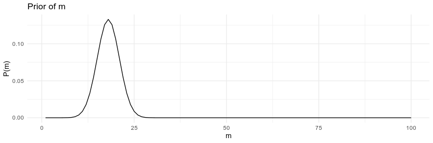
I think one issue with this prior is that it's probably too strong. In the UK, for instance, my tiny Yaris gets 40 mpg easily. If I had collected data in the UK using my prior knowledge from the US, the prior would push me to the wrong answer.

Likelihood

The likelihood is the probability of the data given some parameter values. I got hung up here for some time. None of the books really make it up-front and clear. It wasn't until I saw a post on Cross Validated that I figure out what to do. I had always understood that the likelihood was the observations, but I didn't know how you could transform that into a distribution that could be multiplied by the prior. So here's what we do:

1. Choose two of the parameter values from the grid (the mean and standard deviation)
2. For each value of the data compute the probability using the density function using those two parameter values
3. Multiply all of these probabilities together
4. That's your likelihood probability density estimate for that point in the parameter space, for that pair of the mean and standard deviation

$$f(\mathbf{Y}|\theta)= \prod_{i=1}^n f(y_i|\theta) $$

It seems obvious in retrospect how to do this, but it didn't make sense at first.

mpg_likelihood <- apply(g, 1, FUN = function(r) {
  prod(dnorm(mtcars$mpg, mean = r['m'], sd = r['s']))
})

The R code does exactly what was describe above. It uses the apply function to use each row of the grid table. Then it computes the probability of observing each mpg value we observed if the mean and standard deviation were the values we got from the grid.

Log probabilities

One thing I found was that the probabilities these functions produce were super itty bitty - even using values that were very close to what the actual values were. This presents some difficult problems with floating point arithmetic.

> prod(dnorm(mtcars$mpg, mean = 18, sd = 7))
[1] 3.767108e-46

Which is one of the reasons to use log probabilities. When you use the log probability density the values are far more manageable. You also sum each of values instead of multiplying them (as a consequence of the math of logarithms).

> sum(dnorm(mtcars$mpg, mean = 18, sd = 7, log = TRUE))
[1] -104.5926

However, this isn't explicitly called out in the math of the basic bayesian introductions. I will be doing this from now on, after this experiment.

The Posterior

Now that the likelihood and prior have been computed.... we just multiply them! That creates the unstandardized posterior, then we divide it by the sum of itself. Bam. Posterior.

d <- tibble(m = g$m, s = g$s, 
       mpg_m_prior, mpg_s_prior, mpg_likelihood) %>% 
  mutate(mpg_post_unstd = mpg_m_prior * mpg_s_prior * mpg_likelihood) %>% 
  mutate(post = mpg_post_unstd / sum(mpg_post_unstd))

And here's a visualization of what that looks like. The posterior here is two-dimensional, so I used geom_tile to get  sense of it.

ggplot(d, aes(x = m, y = s, fill = post, z= mpg_post_unstd)) +
  geom_tile() +
  scale_fill_viridis_c() +
  theme_minimal()

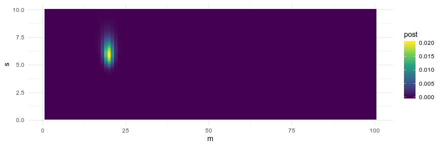
And the Bayesian mean here is 20.

> d[which.max(d$post),]
# A tibble: 1 x 7
      m     s mpg_m_prior mpg_s_prior mpg_likelihood mpg_post_unstd   post
  <dbl> <dbl>       <dbl>       <dbl>          <dbl>          <dbl>  <dbl>
1    20   5.9       0.106        0.05       3.43e-45       1.83e-47 0.0201

The precision of this estimate is restricted by the resolution of the grid. It's exactly 20 because the grid doesn't have values for 20.1 or such.

I increased N to 1000 instead of 100 (thus there were 1,000,000 combinations of parameter values), and I estimated the mean as 19.8.

> d[which.max(d$post),]
# A tibble: 1 x 7
      m     s mpg_m_prior mpg_s_prior mpg_likelihood mpg_post_unstd     post
  <dbl> <dbl>       <dbl>       <dbl>          <dbl>          <dbl>    <dbl>
1  19.8  5.94       0.110        0.05       3.34e-45       1.85e-47 0.000199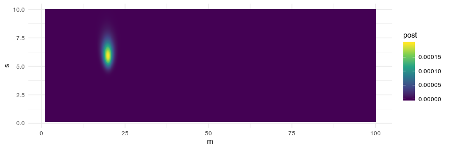

Highest Posterior Density Interval

The posterior is not a point though - it's a distribution. I just used the highest value of the posterior in the grid to select a point value. This gives us some options, do we choose the maximum? - the median? How do we define the credible interval? That's what I wanted to explore in the next post.

[1]: McElreath, R. 2020. Statistical rethinking: A Bayesian course with examples in R and Stan. Boca Raton, FL: Chapman & Hall/CRC Press.

[2]: Gelman, A., Carlin, J. B., Stern, H. S., Dunson, D. B., Vehtari, A., & Rubin, D. B. (2013). Bayesian data analysis. CRC press.

[3]: Kruschke, J. (2014). Doing Bayesian data analysis: A tutorial with R, JAGS, and Stan. Academic Press.